Every once in a while, you need to try an algorithm that’s “custom enough” that it must be coded directly in your “research language”. Perhaps the existing “high-performance” libs don’t support your desired variant or it’s too much setup work switching to another language just to prototype a quick one-off idea. This an instance of the “two language problem” that’s been the reality of technical computing for decades.
Users of R, Python, and similar “high-productivity” environments know that native control flow constructs (for-loops, etc) in those languages kill performance unless they can be expressed in “vectorized” form. One big attraction of Julia to me is that it claims to fix this inconvenience. Let’s have a look.
Preview
- Julia, Python, Java, and C++ are compared for implementing the same iterative algorithm (knapsack solver).
- The implementation does virtually no memory allocation, so what’s being tested is the speed of looping and array access.
- Julia is fast (although not quite as fast as C++ or Java). Python, however, comes out looking horribly slow by comparison.
Benchmark problem
For a simple yet realistic test of performance let’s code a solution to the 0/1 knapsack problem. I am sure you’ve heard of it – it is a classic discrete optimization problem in its own right and shows up as a building block within many optimization algorithms.
As a reminder, the problem is to pack a knapsack of finite weight capacity with a chosen set of items of varying value so as to maximize the total packed value:
\[ \begin{equation*} \begin{aligned} & \underset{x}{\text{maximize}} & & V = \sum_{i=1}^n v_i x_i \\ & \text{subject to} & & \sum_{i=1}^n w_i x_i \leq W \\ & & & x_i \in \{0,1\} \text{ for all } i \text{ in } \{1,\dots,n\} \end{aligned} \end{equation*} \] We have \(n\) items of integral1 weights \(w_i > 0\) and value \(v_i\). \(W\) is the knapsack weight capacity. Each item is either chosen or not, hence the “0/1” in the name.
Since all \(x_i\) are restricted to be binary (boolean), this is an integer linear problem with a search space size of \(2^n\). It can be given to an MILP solver. But because of a simple nested structure the problem also has a straightforward dynamic programming (DP) solution that I can code in a few lines.
Dynamic programming algorithm
Assume the problem has been solved for all knapsack capacities up to some \(w\) while making use of only a subset of items \(1, \dots, j\), and let \(V(w, j)\) be the solution, i.e. the maximum achievable knapsack value. Now consider all smaller subproblems without item \(j\), \(V(w', j-1)\) for all possible \(w'\). \(V(w, j)\) and \(V(w', j-1)\) are connected with a single “move” of looking at item \(j\) and deciding to either include it in the optimal selection for knapsack \(V(w, j)\) or not:
- if including item \(j\) is a move that’s feasible (\(w_j \leq w\)) then \(V(w, j)\) is the best of \(v_j + V(w', j - 1)\) and \(V(w', j - 1)\) depending on whether the move is “optimal” (improves \(V\)) or not; in the former case \(w' = w - w_j\) and in the latter \(w' = w\);
- if including item \(j\) is not feasible (\(w_j > w\)) then \(V(w, j) = V(w', j - 1)\) and \(w' = w\);
- \(V(w, 1)\) is 0 or \(v_1\) depending on whether the first item fits within capacity \(w\).
In other words, knapsack subproblems have a recurrent relationship for \(j > 1\)
\[ V(w, j) = \left\{ \begin{array}{@{}ll@{}} V(w , j - 1) & \text{if}\ w \lt w_j, \\ \max \big\{v_j + V(w - w_j, j - 1),V(w , j - 1)\big\} , & \text{otherwise} \\ \end{array} \right. \] together with a boundary condition for \(j = 1\) \[ V(w, 1) = \left\{ \begin{array}{@{}ll@{}} 0 & \text{if}\ w \lt w_1, \\ v_1, & \text{otherwise} \\ \end{array} \right. \]
(The above could be stated more compactly if \(j\) started at 0 and \(V(w,0)\) were defined as 0.)
To capture inputs into a problem instance, I will use an array of Julia structs. Although I could get away with a list or a tuple, I think a struct makes for more readable example code:
struct Item
    value   ::Int64
    weight  ::Int64
end
If \(V(w, j)\) is represented as a matrix (another first-class citizen in Julia), a non-recursive implementation would be to sweep the space of \(w\) and \(j\) going from smaller to larger item sets:
function opt_value(W ::Int64, items ::Array{Item}) ::Int64
    n = length(items)

    # V[w,j] stores opt value achievable with capacity 'w' and using items '1..j':

    V = Array{Int64}(undef, W, n) # W×n matrix with uninitialized storage

    # initialize first column v[:, 1] to trivial single-item solutions:

    V[:, 1] .= 0
    V[items[1].weight:end, 1] .= items[1].value

    # do a pass through remaining columns:

    for j in 2 : n
        itemⱼ = items[j]
        for w in 1 : W
            V_without_itemⱼ = V[w, j - 1]
            V_allow_itemⱼ = (w < itemⱼ.weight
                ? V_without_itemⱼ
                : (itemⱼ.value + (w ≠ itemⱼ.weight ? V[w - itemⱼ.weight, j - 1] : 0)))
            V[w, j] = max(V_allow_itemⱼ, V_without_itemⱼ)
        end
    end

    return V[W, n]
end
That loop is almost a straightforward translation of my recurrence, although the body needs some extra edge condition checks. Note the familiar ?: syntax for ternary operator and some comforting exploitation of Julia’s support for Unicode math symbols.
This may not be the best bit of Julia code you’ll ever see, but I’ve literally just learned enough syntax for my first experiment here. One performance-related concession to Julia has already been included above by arranging to traverse \(V\) in column-major order. Yes, Julia opts for R/MATLAB/Fortran design choice here and that is not under end user control, as far as I can tell at this point. Right now, it does feel like R and yet awkwardly different from C++, which would be my production choice for this particular problem.
An obvious improvement
Notice also that I cheat a little and do not compute half of the solution, specifically the optimal \(x_i\)’s2. This is to keep the experiment simple and focus on iterative performance only. However, since this means I don’t need to capture the optimal solution structure in \(V\) matrix, I don’t need to allocate it: it is sufficient to allocate a couple of buffers for columns \(j\) and \(j-1\) and re-use them as needed:
function opt_value(W ::Int64, items ::Array{Item}) ::Int64
    n = length(items)

    V = zeros(Int64, W) # single column of size W, zero-initialized
    V_prev = Array{Int64}(undef, W) # single column of size W, uninitialized storage

    V[items[1].weight:end] .= items[1].value

    for j in 2 : n
        V, V_prev = V_prev, V
        itemⱼ = items[j]
        for w in 1 : W
            V_without_itemⱼ = V_prev[w]
            V_allow_itemⱼ = (w < itemⱼ.weight
                ? V_without_itemⱼ
                : (itemⱼ.value + (w ≠ itemⱼ.weight ? V_prev[w - itemⱼ.weight] : 0)))
            V[w] = max(V_allow_itemⱼ, V_without_itemⱼ)
        end
    end

    return V[W]
end
This version will now scale to quite large problem instances.
Algorithm speed: Julia vs Python vs Java vs C++
To measure performance, I use the @elapsed macro from Julia’s family of @time and friends with randomly constructed problem instances of different scale. Because Julia is JIT-based I need to be careful and do a few timing repeats after burning the very first measurement.
Actually, I’ll use the median of 5 repeats which is even more robust:
function run(repeats = 5)
    @assert repeats > 1

    times = zeros(Float64, repeats)
    seed = 12345

    for W in [5_000, 10_000, 20_000, 40_000, 80_000]
        for repeat in 1 : repeats
            spec = make_random_data(W, seed += 1)
            times[repeat] = @elapsed opt_value(spec[1], spec[2])
        end
        sort!(times)
        println(W, ", ", times[(repeats + 1) ÷ 2])
    end
end
For the promised language shootout, I’ve implemented this same algorithm in three other languages: Python, Java, and C++. I event went as far as make sure that all “ports” used similar array data types and even the exact same random number generator for building the exact same random problem instances. To maintain consistency with statically typed languages (Java, C++), I ensure that value types used by the dynamic versions are 64-bit integers as much as possible – this required some minor contortions in Python.
Here’s the C++ version of opt_value() (you can get all four language versions from this github repo, there is a single source file per language that’s trivial to compile and run):
int64_t
opt_value (int64_t const W, std::vector<item> const & items)
{
    auto const n = items.size ();

    std::unique_ptr<int64_t []> const v_data { std::make_unique<int64_t []> (W) }; // "zeros"
    std::unique_ptr<int64_t []> const v_prev_data { std::make_unique<int64_t []> (W) }; // "zeros"

    int64_t * V { v_data.get () };
    int64_t * V_prev { v_prev_data.get () };

    for (int64_t w = items[0].weight; w <= W; ++ w)
        V[w - 1] = items[0].value;

    for (std::size_t j = 1; j < n; ++ j)
    {
        std::swap (V, V_prev);
        item const & item { items [j] };

        for (int64_t w = 1; w <= W; ++ w)
        {
            auto const V_without_item_j = V_prev[w - 1];
            auto const V_allow_item_j = (w < item.weight
                ? V_without_item_j
                : (item.value + (w != item.weight ? V_prev[w - 1 - item.weight] : 0)));

            V[w - 1] = std::max(V_allow_item_j, V_without_item_j);
         }
    }

    return V[W - 1];
}
I’ve tried to keep the implementation consistent and idiomatic within each language. (It helps that my algorithm is basically a couple of nested loops without memory allocation, some arithmetic, and not much else.) All these implementations could in principle be tuned further using language-specific techniques, but that’s not my goal here.
Here is a snippet of calculation latency data for \(W=80000\), captured on the exact same CPU:
| lang | W | time (sec) |
|---|---|---|
| julia | 80000 | 0.1135 |
| python | 80000 | 28.2094 |
| java | 80000 | 0.0781 |
| c++ | 80000 | 0.0710 |
Hmm. Perhaps you begin to suspect that Python is not going to win this. Here is a log-log plot of all data, for all \(W\)’s:
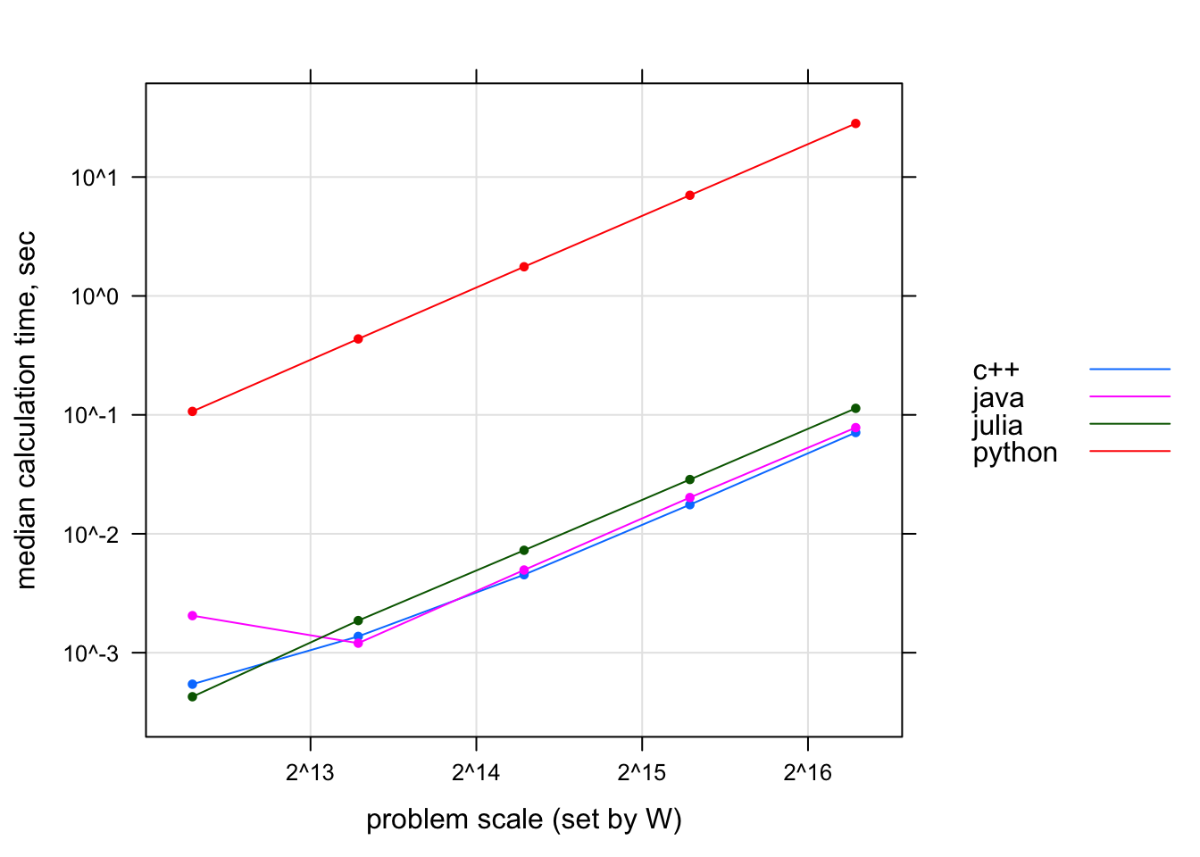
Figure 1: Calculation time as a function of knapsack problem size. (Note that both axes use log scale.)
Julia is about 50% slower than either Java or C++. But it is Python that is the real laggard in the group: slower by more than 100x across the entire range of tested problem sizes. Ouch!
Going back to the matrix version of the algorithm, you can see how the matrix is accessed predictably over \(j\) columns but somewhat randomly (in a data-depedent fashion) over \(w\) rows. There doesn’t seem to be a way to express the algorithm in linear algebra operations. This difficulty is retained in the optimized two-column-buffer version. The algorithm is short and simple but there just doesn’t seem to be a way to vectorize it so that it would be fast, say, in numpy. Massive underperformance of the Python version is the cost I pay for slow interpretation of Python bytecode.
As for Julia, so far so good. I might just get used to the “no need to vectorize code to make it fast” lifestyle.